Fabric end-to-end use case: Analytics Engineering part 1 - dbt with the Lakehouse

26 minutes

September 11, 2023

MICROSOFT FABRIC, ANALYTICS ENGINEERING, DATA LAKEHOUSE, DBT, SQL, PYTHON

Welcome to the fourth part of a 5-part series on an end-to-end use case for Microsoft Fabric. This post will focus on the analytics engineering part of the use case.

In this series, we will explore how to use Microsoft Fabric to ingest, transform, and analyze data using a real-world use case. The series focuses on data engineering and analytics engineering. We will be using OneLake, Notebooks, Lakehouse, SQL Endpoints, Data Pipelines, dbt, and Power BI.

All posts in this series

This post is part of a 5-part series on an end-to-end use case for Microsoft Fabric:

Use case introduction: the European energy market

If you’re following this series, feel free to skip this section as it’s the same introduction every time. 🙃

Since Russia invaded Ukraine, energy prices across Europe have increased significantly. This has led to a surge of alternative and green energy sources, such as solar and wind. However, these sources are not always available, and the energy grid needs to be able to handle the load.

Therefore, most European energy markets are converging towards a model with dynamic energy prices. In a lot of European countries, you can already opt for a dynamic tariff where the price of electricity changes every hour. This brings challenges, but also lots of opportunities. By analyzing the prices, you can optimize your energy consumption and save money. The flexibility and options improve a lot with the installation of a home battery. With some contracts, you could even earn money by selling your energy back to the grid at peak times or when the price is negative.

In this use case, we will be ingesting Epex Spot (European Energy Exchange) day-ahead energy pricing data. Energy companies buy and sell energy on this exchange. The price of energy is announced one day in advance. The price can even become negative when there will be too much energy on the grid (e.g. it’s sunnier and windier than expected and some energy plants cannot easily scale down capacity).

Since it’s quite a lot of content with more than 1 hour of total reading time, I’ve split it up into 5 easily digestible parts.

We want to ingest this data and store it in OneLake. At one point, we could combine this data with weather forecasts to train a machine learning model to predict the energy price.

After ingestion, we will transform the data and model it for dashboarding. In the dashboard, we will have simple advice on how to optimize your energy consumption and save money by smartly using a home battery.

All data is publicly available, so you can follow along in your own Fabric Workspace.

Why dbt? And how?

dbt is a popular open-source analytics engineering tool that allows you to transform data in your warehouse. I helped build dbt support for Microsoft Fabric, and I’m excited to show you how it works. If you want to learn more about dbt itself, check out my other posts about dbt .

dbt is a great fit for this use case as we want to transform the raw relational electricity pricing data into data marts ready for visualization through Power BI. It has the advantage that everything we build can be stored in git and includes great data lineage and documentation features.

Note that in this blog post and use case, we will be using dbt with a Lakehouse on Fabric. The Lakehouse works great with dbt, but only exposes a small subset of dbt’s capabilities. If you want to use dbt to the fullest, you can use it with a Fabric Data Warehouse.

In this post we’ll take our first steps with dbt and we’ll also look at the best practices on using dbt. dbt itself is a very simple tool, but the power comes from how you use it.

Installing dbt-fabric

dbt is a Python package, so make sure you have Python installed and create a new project folder on your machine. I’d suggest creating a virtual environment for your project, but that’s not required. Open a terminal and run the following commands:

1mkdir fabric-epex
2cd fabric-epex
3python -m venv .venv

The syntax for activating the virtual environment differs between operating systems and shells.

OS	Shell	Command to activate virtual environment
Windows	cmd.exe	`.venv\Scripts\activate.bat`
Windows	PowerShell	`.venv\Scripts\Activate.ps1`
macOS/Linux	bash/zsh	`source .venv/bin/activate`
macOS/Linux	PowerShell	`.venv/bin/Activate.ps1`

Once you have activated your virtual environment, you can install dbt with Fabric support.

1pip install dbt-fabric

There is one more requirement we need to fulfill: the ODBC driver. Connections to Fabric go over either TDS or ODBC. For dbt, we need the ODBC driver. You can find the installation instructions here .

Tooling: VS Code

Since Fabric support is not available on dbt Cloud yet, I’d recommend to use Visual Studio Code to work with dbt projects at the moment. In VS Code, you can configure the IDE to use the Python interpreter from the virtual environment you created above. If you then open new terminal windows in VS Code, they will automatically have the virtual environment activated.

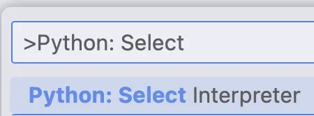
If you open the Command Palette in VS Code, you can look for Python: Select to configure the Python interpreter and select the one from your virtual environment.

Selecting the Python interpreter in VS Code

Authentication

There are lots of ways to authenticate to Fabric from dbt, but the easiest one is probably to use the Azure CLI. If you don’t have it installed yet, you can find instructions here .

Once you have the Azure CLI installed, you can log in with the command az login. This will open a browser window where you can log in with your Azure credentials.

Creating a dbt project

Now that you have dbt installed and are authenticated to Fabric, you can create a new dbt project. Run the following command in your terminal:

1dbt init fabric_epex

Project names in dbt cannot have dashes, so we’re using an underscore in the name above. dbt will ask you which adapter you want to use, but at this point, the one for Fabric is the only one you have installed, so you can just press enter.

Configuring the dbt profile

Profiles in dbt are used to store connection details and credentials to your data warehouse. The default location for dbt profiles is in your home directory. Since we’re using Azure CLI for authentication, we have the benefit that our profile will not contain any credentials by itself. That means we can store it right in our dbt project folder and commit it to git.

Create a new file called profiles.yml in the fabric_epex folder and add the following content:

 1fabric_epex:
 2  target: dev
 3  outputs:
 4    dev:
 5      type: fabric
 6      driver: ODBC Driver 18 for SQL Server
 7      server: connection_string_from_fabric # change this
 8      port: 1433
 9      authentication: cli
10      database: name_of_your_lakehouse # change this
11      schema: dbo

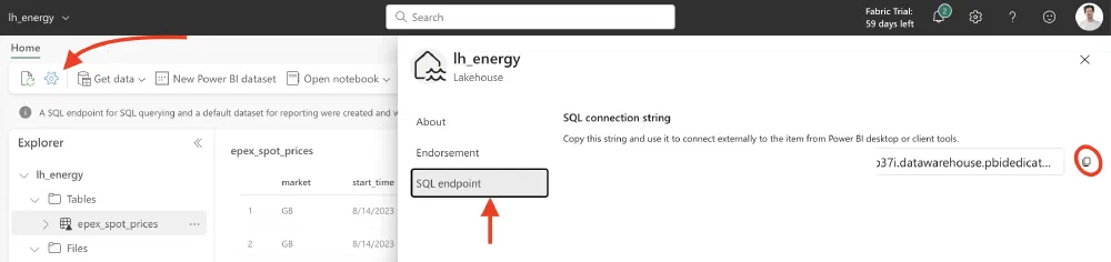
As you can see from the snippet above, there are two things you need to change: the connection string and the database name. The name of the lakehouse is an easy one, but for the connection string, you need to know where to look. Navigate to your Lakehouse, click on the ⚙️ settings icon and then on SQL endpoint. Here, you can copy your connection string.

You can validate that your configuration is working by running the command dbt debug in the terminal where you have your virtual environment activated.

Deleting sample data and configuration

New dbt projects come with sample data and configuration. We don’t need any of that, so delete the contents of the models folder and replace the dbt_project.yml file with the following:

1name: 'fabric_epex'
2version: '1.0.0'
3config-version: 2
4
5profile: 'fabric_epex'
6
7models:
8  fabric_epex:
9    +materialized: view

Since the Lakehouse can only create SQL Views and not Tables (only through Spark), we configure the project to materialize all models as views. In future dbt blog posts , I’ll go deeper into the different materializations and how they work in Fabric.

Creating the first model and source

A model in dbt is a SQL query that transforms data. It takes the form of a SQL file containing a SELECT statement. dbt then materializes the output of the query as views, tables, or CTEs. In our case, we want to create a view that transforms the raw data from the Lakehouse into data marts.

What is a CTE?

A CTE is a Common Table Expression. It’s a way to split up a SQL query into multiple logical parts. You can think of it as a temporary table that only exists for the duration of the query. It’s a great way to make your SQL code more readable and maintainable. You could probably write more performant queries without CTEs, but that’s not the goal of dbt. It’s meant to make your code more readable, understandable, and maintainable. If an analytics query takes 5 minutes instead of 4, that’s not a big of a deal since they are usually run once or a couple of times a day.

Staging source

Create a folder named staging in the models folder. This is where we will put the models that load the raw data from the Lakehouse. We only have 1 raw table, so we only need 1 raw model. For our model to be able to reference this table, we have to define the table as a source.

Create a file called __sources.yml in the staging folder you just created. You can name the file itself however you’d like, but I prefer the double underscore to make sure that I can easily find the file at top of the folder. Add the following content to the file:

 1version: 2
 2
 3sources:
 4  - name: epex_spot_prices
 5    schema: dbo
 6    tables:
 7      - name: epex_spot_prices
 8        description: The EPEX Spot prices for the day-ahead market
 9        columns:
10          - name: market
11            description: The market for which this price is valid
12          - name: start_time
13            description: The timestamp this price becomes valid
14          - name: end_time
15            description: The timestamp this price is no longer valid
16          - name: buy_volume
17            description: The volume of buy orders at this price (in MWh)
18          - name: sell_volume
19            description: The volume of sell orders at this price (in MWh)
20          - name: volume
21            description: The total trading volume of orders at this price (in MWh)
22          - name: price
23            description: The energy price (in EUR/MWh)

So as you can see, we tell dbt the name of the schema and the table where it can find our source data. We also define all columns and give descriptions for each column. This is how you document your data in dbt. You’ll see in a bit how this documentation can be used and visualized.

This source by itself doesn’t do anything. You can validate this by running dbt run in your terminal, it will output Found 0 models, 0 tests, 0 snapshots, 0 analyses, 327 macros, 0 operations, 0 seed files, 1 source, 0 exposures, 0 metrics. That means that it found our source, so now we can create a model that references it.

Staging model

Create a new file called stg_epex_spot_prices.sql in the same staging folder and add the following content:

 1with src as (
 2    select *
 3    from {{ source('epex_spot_prices', 'epex_spot_prices') }}
 4),
 5
 6conversions as (
 7    select
 8        market,
 9        convert(date, start_time) as date,
10        convert(time, start_time) as start_time,
11        convert(time, end_time) as end_time,
12        price / 10 as price_cent_kwh
13    from src
14),
15
16with_country as (
17    select
18        *,
19        case
20            when market like 'NO%' then 'Norway'
21            when market like 'SE%' then 'Sweden'
22            when market like 'DK%' then 'Denmark'
23            when market like 'DE-LU' then 'Germany'
24            when market = 'FI' then 'Finland'
25            when market = 'BE' then 'Belgium'
26            when market = 'PL' then 'Poland'
27            when market = 'AT' then 'Austria'
28            when market = 'FR' then 'France'
29            when market = 'NL' then 'the Netherlands'
30            when market = 'CH' then 'Switzerland'
31            when market = 'GB' then 'United Kingdom'
32            else 'Unknown'
33        end as country
34    from conversions
35),
36
37final as (
38    select
39        *,
40        case
41            when country in ('Belgium', 'the Netherlands', 'Germany', 'France', 'Switzerland', 'Austria') then 'West Europe'
42            when country in ('Great Britain') then 'North Europe'
43            when country in ('Poland') then 'Central Europe'
44            when country in ('Norway', 'Sweden', 'Finland', 'Denmark') then 'Scandinavia'
45            else 'Unknown'
46        end as region
47    from with_country
48    where price_cent_kwh > 0
49)
50
51select
52    market,
53    date,
54    start_time,
55    end_time,
56    price_cent_kwh,
57    country,
58    region
59from final

There a few dbt best practices you can see being applied here:

Split all the transformations into CTEs. This makes it easier to read and understand the code.
The last CTE should be named final and the last SELECT statement should select from final. This makes it easier to find the output of the model and to add more CTEs later on.
Use the source macro to reference the source table. This makes it easier to change the source table later on. This also tells dbt how dependencies work in your project and will become visible in the documentation.
Don’t do any major transformations in the staging models themselves. They are meant to cleanse, but not to end up with a completely different table structure.
Always expose the raw source data in the staging models. This makes it easier to debug and to understand the data lineage.

The SQL itself is pretty straightforward, but if you’re new to dbt, then this will be the first time you’re seeing Jinja in {{ source('epex_spot_prices', 'epex_spot_prices') }}. This is the source macro I mentioned above. It takes the name of the source and the name of the table and returns the fully qualified name of the table. In this case, it will return name_of_your_lakehouse.dbo.epex_spot_prices. This way you can decouple the source name from the actual table name.

The first run

Nothing more exciting than the first succeeding dbt run 😊. Run dbt run in your terminal and you should see the command succeeding with the message Completed successfully followed by Done. PASS=1 WARN=0 ERROR=0 SKIP=0 TOTAL=1.

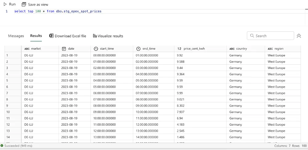
You can look at your fancy new dbt model in the Lakehouse UI on Fabric as well.

The materialized dbt model in the Lakehouse UI

This also compiled our code. You can find the output of the compilation in the target folder, under the subfolder compiled. There, dbt follows the same structure as your project and puts the compiled SQL files. You can find the compiled SQL for our model in target/compiled/fabric_epex/staging/stg_epex_spot_prices.sql. In this compiled version, the Jinja was replaced by the actual value. This is what dbt used to build the view in the Lakehouse.

Generating documentation

We already added some documentation to our source, but we can do better by also properly documenting our dbt model. Like with the source definition, you can name the yaml file however you’d like, but I prefer __schema.yml to keep it a the top of the folder.

This is what I’ve put inside the file:

 1version: 2
 2
 3models:
 4  - name: stg_epex_spot_prices
 5    description: The EPEX Spot prices for the day-ahead market
 6    columns:
 7      - name: market
 8        description: The market for which this price is valid
 9      - name: date
10        description: The date this price becomes valid
11      - name: start_time
12        description: The timestamp this price becomes valid
13      - name: end_time
14        description: The timestamp this price is no longer valid
15      - name: price_cent_kwh
16        description: The energy price (in euro cent/kWh)
17      - name: country
18        description: The country in which this market is located
19      - name: region
20        description: Where in Europe the market is located

Now, run dbt docs generate in your terminal. This will generate the documenation as a static HTML website in a folder called target. To open the documentation in your browser automatically, you can run dbt docs serve.

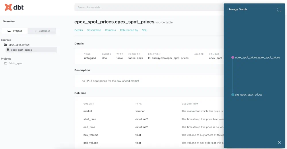
From there, you can navigate through the project and open the source and the model to see their documentation. It includes descriptions of the table, the view, the columns, the code used, references, and much more. If we click the Lineage graph button in the bottom right corner, we can see the data lineage of our model. This is a pretty simple one, since we only have 1 source and 1 model, but it will grow as we add more models.

The dbt documentation and the lineage information

Side note: modelling

Experienced data analysts will notice that I’m not using the Kimball model in this use case. Instead, I opted for OBT: One Big Table. Every data mart will be a table with all the information in it. This is not a requirement for dbt or for the Lakehouse and not a recommendation either. You can model your data however you’d like and I felt most comfortable with this approach for this use case. But you could easily use the Kimball model as well.

Building data marts

Now that we have our source data available in a model, we can start building data marts on top of it. Create a new folder named marts in the models folder. We’ll create the markets below one by one. During this process, make sure to run dbt run after each change to validate that your code compiles and runs successfully.

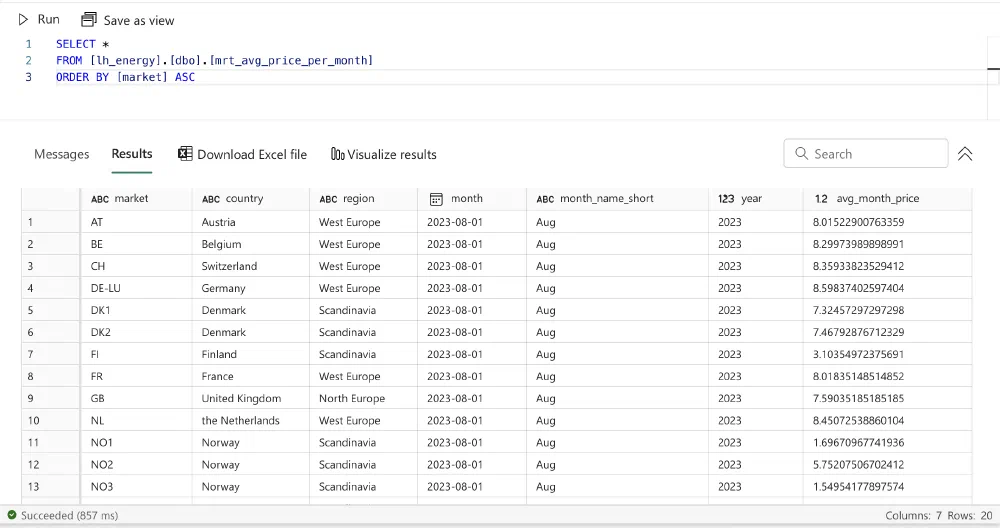
Data mart: average price per month per market

Let’s start simple and create a mart that calculates the average price per month per market. Create a new file called mrt_avg_price_per_month.sql in the marts folder and add the following content:

 1with stg as (
 2    select *
 3    from {{ ref('stg_epex_spot_prices') }}
 4),
 5
 6with_month as (
 7    select
 8        *,
 9        datetrunc(month, date) as month,
10        year(date) as year,
11        format(date, 'MMM') as month_name_short
12    from stg
13),
14
15final as (
16    select
17        market,
18        country,
19        region,
20        month,
21        month_name_short,
22        year,
23        avg(price_cent_kwh) as avg_month_price
24    from with_month
25    group by market, country, region, month, month_name_short, year
26)
27
28select *
29from final

There are a few things we can observe in this SQL query:

We use the ref macro to reference the staging model. This is the same as the source macro, but it’s used for models instead of sources. Since we can have multiple sources, but only one dbt project (this is changing in dbt 1.6), we only have to specify the name of the model that we’re referencing. The model can be located in any folder and can be materialized as anything. We could even configure the referenced model to have a different schema or view name in the Lakehouse and our reference would still work.
The referenced model is the first CTE in the query. It’s a best practice to put all the models you’re referencing as 1:1 CTEs as the top of the model. This makes it easier to the reader of your code to understand where the data is coming from.
Besides the reference, we have 2 CTEs. We have the final one, as in our previous model, and we have one where we add information about the month to the data. In the final CTE, we group all columns by the month and the market and calculate the average price per month per market.

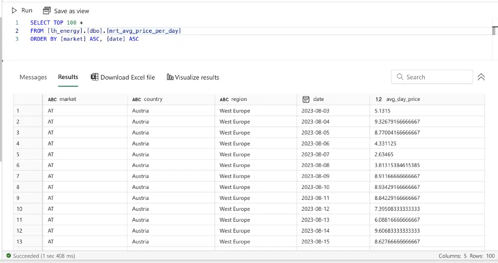
Data mart: average price per day per market

Let’s create another data mart that calculates the average price per day per market. Create a new file called mrt_avg_price_per_day.sql in the marts folder and add the following content:

 1with stg as (
 2    select *
 3    from {{ ref('stg_epex_spot_prices') }}
 4),
 5
 6final as (
 7    select
 8        market,
 9        country,
10        region,
11        date,
12        avg(price_cent_kwh) as avg_day_price
13    from stg
14    group by market, country, region, date
15)
16
17select *
18from final

This one is much simpler than the previous one. We don’t need to add any information about the date, since we’re grouping by the date itself. We can just calculate the average price per day per market.

Data mart: transposed version of the average price per day per market

Now, let’s try something more challenging where we can also start to see the value of dbt a bit more. We want to create a data mart that has the average price per day per market, but transposed. So instead of having 1 row per day per market, we want to have 1 row per day with a column for each market.

Create a new file called mrt_avg_price_per_day_transposed.sql in the marts folder and add the following content:

 1{% set markets_query %}
 2    select
 3        distinct market
 4    from {{ ref('stg_epex_spot_prices') }}
 5    order by market
 6{% endset %}
 7
 8{% set markets_query_results = run_query(markets_query) %}
 9
10{% if execute %}
11    {% set markets = markets_query_results.columns[0].values() %}
12{% else %}
13    {% set markets = [] %}
14{% endif %}
15
16with avgs as (
17    select *
18    from {{ ref('mrt_avg_price_per_day') }}
19),
20
21final as (
22    select
23        date,
24        {% for market in markets %}
25        sum(
26            case
27                when market = '{{ market }}' then avg_day_price
28                else 0
29            end
30        ) as market_{{ market | replace("-","_") | lower }}
31        {% if not loop.last %},{% endif %}
32        {% endfor %}
33    from avgs
34    group by date
35)
36
37select *
38from final

We can build upon the previous data mart. We could have opted to keep our data lineage a bit simpler and follow another dbt best practice by having an intermediate model in between. What’s that? We’d move the contents of the model with the average price per day into a different model in a folder named intermediate and then reference that model in the data mart as well as in this model. Given that this is a small project, I opted to keep it simple and just reference the data mart directly.

We can distinguish the 2 CTEs at the bottom, but the more interesting part is at the top. We want to create one column per market, so in our final CTE we’d have to iterate over all markets.

Variables in Jinja

Most of the Jinja statements we saw until now have double curly braces {{ funtion_name() }} which means that you’re outputting something. In Jinja, you’ll also often notice a curly brace with a percentage sign {% operation %}. This means that you’re executing something. Here, you can implement logical and conditional statements.

A common operation is to set a variable, just like you’d in Python. To set a variable, begin you statement with the set keyword. In the first lines of the query we create a variable named markets_query and set its content to the SQL query on lines 2 to 5, ending with the endset keyword. This is called a multi-line set statement. Right below, on line 8, we see a single-line set statement. Here, we set the value of the variable markets_query_results to the result of the query we just defined. This means that dbt will have to execute the query on lines 2 to 5 and store the result in the variable.

Compilation and execution

There is an important remark to take into account here. dbt has 2 stages: compilation and execution. In the compilation stage, it takes all the dbt models and compiles the Jinja-SQL into regular SQL. In the execution stage, it runs the compiled SQL against the configured data warehouse; in this case the Lakehouse. You can compile your code with the command dbt compile. This creates the artifacts in the target folder mentioned above. This means that only during the execution phase, dbt runs queries against the Lakehouse. That is why we have a conditional statement in the code above. We only want to execute the query if we’re in the execution phase. If we’re in the compilation phase, we don’t want to run the query and we just set it to an empty list.

Loops in Jinja

This all comes together in lines 24 to 32. Here we use a for loop to iterate over all the markets present in our data. We then use a CASE statement in SQL to create a column for each market. Since the market names can contain dashes, we replace them with underscores and convert the whole string to lowercase to have consistent column names. Let’s also have a closer look at line 28. Columns in a SELECT statement are separated by commas, but we can’t have a comma after the last column. So we use the special loop variable in dbt to check if we’re at the last iteration of the loop. If we are, we don’t add a comma, otherwise we do.

Putting it all together

We then group by the date column to have a single row per date and summarize the average price per market in the columns we created. This is the result:

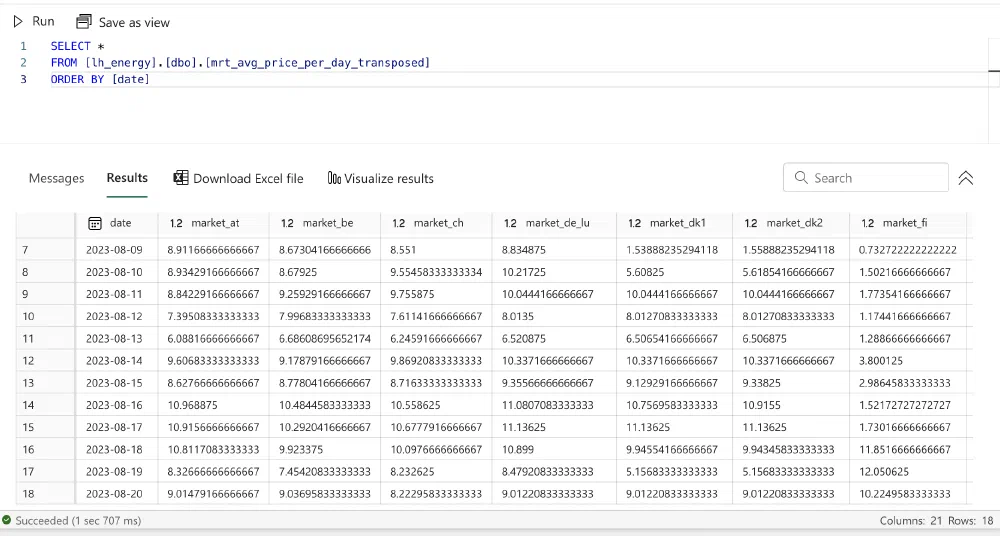
Without dbt’s powerful Jinja syntax, we’d have to write a lot more SQL, with a few lines of code per market, to achieve the same result.

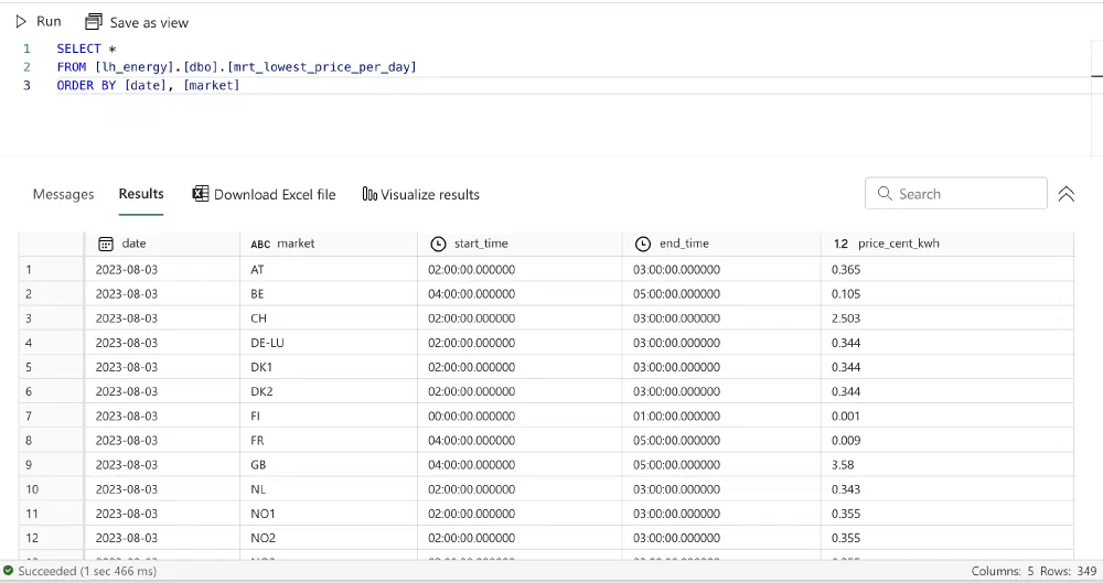
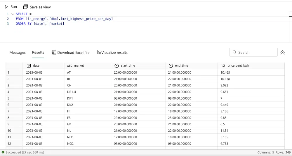
Data marts: lowest and highest price per day per market

Next, I’d like to have 2 more data marts that show me the moment of the lowest price per day and the moment of highest price per day for each market. Let’s start with the lowest price. Create a new file called mrt_lowest_price_per_day.sql in the marts folder and add the following content:

 1with stg as (
 2    select
 3        market,
 4        date,
 5        start_time,
 6        end_time,
 7        price_cent_kwh
 8    from {{ ref('stg_epex_spot_prices') }}
 9),
10
11with_rank as (
12    select
13        *,
14        row_number() over (partition by date, market order by price_cent_kwh asc) as rn
15    from stg
16),
17
18final as (
19    select
20        date,
21        market,
22        start_time,
23        end_time,
24        price_cent_kwh
25    from with_rank
26    where rn = 1
27)
28
29select *
30from final

This is again a pretty straightforward SQL query, following the best practices as outlined in the previous dbt models. We’re using a windowing function to rank the prices per day per market from lowest to highest and then take the rows with the lowest ranks/prices.

Now, for the highest price, the only difference is that we order by the price descending instead of ascending. It seems a bit silly to just copy the entire file and change 3 characters. Luckily, dbt has a solution that allows us to make our code more flexible.

Creating macros

Macros are reusable bits of SQL code that can parametrized. You could think of them like functions in Python. You can use any SQL or Jinja in a macro. Let’s see how this works with our example.

Start by creating a file named find_date_moment.sql in the macros folder in your project. Add the following content:

 1{% macro find_date_moment(which_moment) %}
 2    {% set order = "asc" %}
 3    {% if which_moment == "highest" %}
 4        {% set order = "desc" %}
 5    {% endif %}
 6
 7    with stg as (
 8        select
 9            market,
10            date,
11            start_time,
12            end_time,
13            price_cent_kwh
14        from {{ ref('stg_epex_spot_prices') }}
15    ),
16
17    with_rank as (
18        select
19            *,
20            row_number() over (partition by date, market order by price_cent_kwh {{ order }}) as rn
21        from stg
22    ),
23
24    calc_result as (
25        select
26            date,
27            market,
28            start_time,
29            end_time,
30            price_cent_kwh
31        from with_rank
32        where rn = 1
33    )
34{% endmacro %}

A macro is created with the macro and endmacro keywords within {% and %}. Our macro takes 1 argument named which_moment to indicate if we want to find the moments with the lowest or the highest price. Then we change the order accordingly on lines 2 to 5 by setting a variable named order to the corresponding value. We have to parametrize the ordering on line 20, so there we can use our order variable.

Using macros

Using macros work in the exact same way as how we used the built-in ref and source macros. We can just call our macro with double curly braces like so: {{ find_date_moment("highest") }}. Let’s change the content of our mrt_lowest_price_per_day.sql file to the following:

1{{ find_date_moment("lowest") }}
2
3select * from calc_result

And then we can create our second data mart named mrt_highest_price_per_day.sql with the following content:

1{{ find_date_moment("highest") }}
2
3select * from calc_result

You’ll notice the first data mart still produces exact the same output and our second data mart works flawlessly as well.

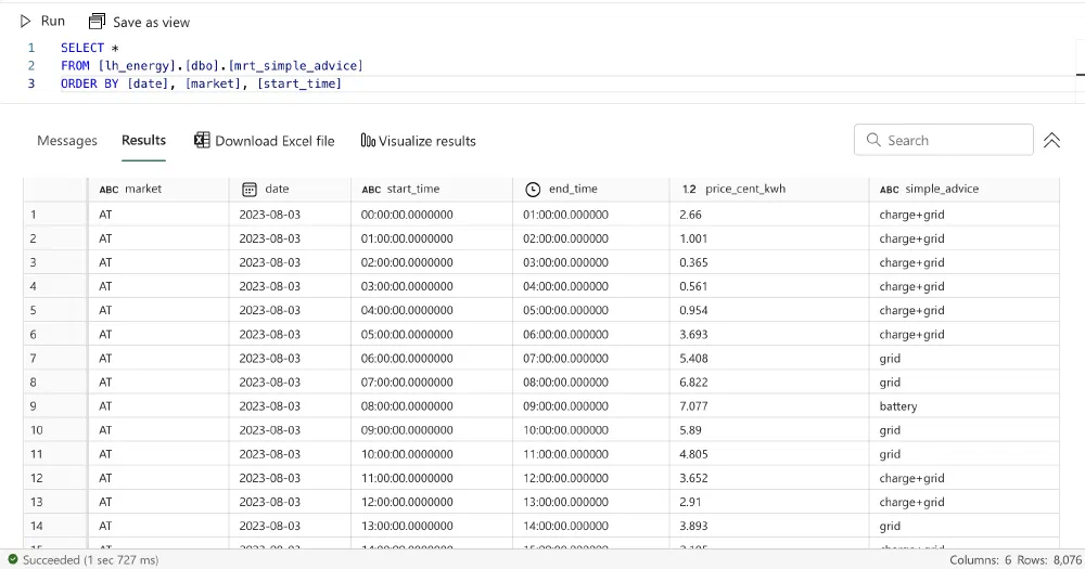
Data mart: simple advice

Our final data mart is a simple one. The goal of this data mart is to provide some very basic advice to electricity consumers with a home battery. If you intelligently use your home battery by charging it when the price is low and discharging it when the price is high, you can save money. In some countries you could even make money by selling your electricity back to the grid when the price is high if you charge your battery when the price is low.

This is under no circumstances financial advice and also not super reliable. This is just meant as an example to showcase what you could do with this data.

Create a new file called mrt_simple_advice.sql in the marts folder and add the following content:

 1{{ find_date_moment("lowest") }}
 2
 3, final as (
 4    select
 5        market,
 6        date,
 7        substring(convert(nvarchar, start_time, 14), 1, 5) as start_time,
 8        substring(convert(nvarchar, end_time, 14), 1, 5) as end_time,
 9        price_cent_kwh,
10        case
11            when price_cent_kwh < 0 then 'discharge'
12            when rn < 10 then 'charge+grid'
13            when rn < 18 then 'grid'
14            when rn < 24 then 'battery'
15            else 'battery+discharge'
16        end as simple_advice
17    from with_rank
18)
19
20select *
21from final

As you can see, we can reuse our macro ranking the prices per day per market. The macro outputs a CTE with all the ranks, so we can just use that CTE in our final CTE. Depending on the rank, we then output a simple advice.

If the price is negative, we advise to discharge the battery to make some profit. If the price is in the lowest 10 prices for that day, we advise to charge the battery and consume electricity from the grid. For the next 8 pricing moments (ascending), we advise to consume electricity from the grid, without consuming electricity from the battery. For all other pricing moments except for the highest price throughout the day, we recommend to only consume electricity from the battery. Finally, on the most expensive moment of the day, we even recommend to discharge the battery to make some profit.

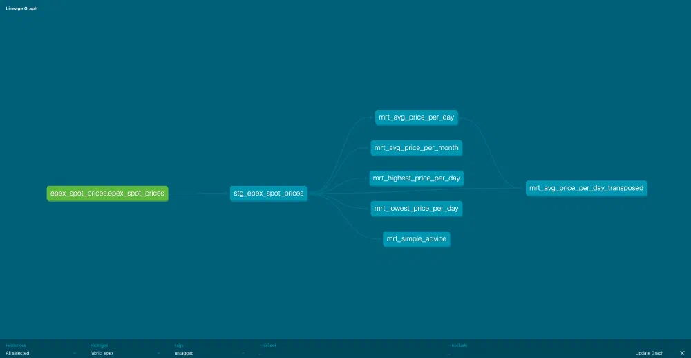
The simple electricity consumption advice data mart

Lineage

Now that our project is finished, we can also take a look at the end result of the lineage. If you run dbt docs generate again, followed by dbt docs serve, you can open the entire Lineage graph by clicking the Lineage button on the bottom right corner.

Finished source code

This concludes our dbt project to build data marts on top of the raw data from the Lakehouse. You can find the finished dbt project here, on GitHub .

👉 Next part

In the next part, we’ll use our data marts in a Report to visualize their output.

The link will start working as soon as the post is published, about a week after this one.

If you liked this article, follow me on LinkedIn or other social media to stay up-to-date with my latest posts. You might also like the following 2 posts about related topics:

Fabric end-to-end use case: overview & architecture

6 minutes

August 21, 2023

Fabric end-to-end use case: overview & architecture

Welcome to the first part of a 5-part series on an end-to-end use case for Microsoft Fabric. This post will focus on the architecture overview of the use case. In this series, we will explore how to use Microsoft Fabric to ingest, transform, and analyze data using a real-world use case.

Fabric end-to-end use case: Data Engineering part 1 - Spark and Pandas in Notebooks

13 minutes

August 28, 2023

Fabric end-to-end use case: Data Engineering part 1 - Spark and Pandas in Notebooks

Welcome to the second part of a 5-part series on an end-to-end use case for Microsoft Fabric. This post will focus on the data engineering part of the use case. In this series, we will explore how to use Microsoft Fabric to ingest, transform, and analyze data using a real-world use case.

Sam Debruyn

Cloud Data Solution Architect