Fabric end-to-end use case: Data Engineering part 1 - Spark and Pandas in Notebooks

Welcome to the second part of a 5-part series on an end-to-end use case for Microsoft Fabric. This post will focus on the data engineering part of the use case.

In this series, we will explore how to use Microsoft Fabric to ingest, transform, and analyze data using a real-world use case. The series focuses on data engineering and analytics engineering. We will be using OneLake, Notebooks, Lakehouse, SQL Endpoints, Data Pipelines, dbt, and Power BI.

All posts in this series

This post is part of a 5-part series on an end-to-end use case for Microsoft Fabric:

• Fabric end-to-end use case: overview & architecture
• Fabric end-to-end use case: Data Engineering part 1 - Spark and Pandas in Notebooks
• Fabric end-to-end use case: Data Engineering part 2 - Pipelines
• Fabric end-to-end use case: Analytics Engineering part 1 - dbt with the Lakehouse
• Fabric end-to-end use case: Analytics Engineering part 2 - Reports

Use case introduction: the European energy market

If you’re following this series, feel free to skip this section as it’s the same introduction every time. 🙃

Since Russia invaded Ukraine, energy prices across Europe have increased significantly. This has led to a surge of alternative and green energy sources, such as solar and wind. However, these sources are not always available, and the energy grid needs to be able to handle the load.

Therefore, most European energy markets are converging towards a model with dynamic energy prices. In a lot of European countries, you can already opt for a dynamic tariff where the price of electricity changes every hour. This brings challenges, but also lots of opportunities. By analyzing the prices, you can optimize your energy consumption and save money. The flexibility and options improve a lot with the installation of a home battery. With some contracts, you could even earn money by selling your energy back to the grid at peak times or when the price is negative.

In this use case, we will be ingesting Epex Spot (European Energy Exchange) day-ahead energy pricing data. Energy companies buy and sell energy on this exchange. The price of energy is announced one day in advance. The price can even become negative when there will be too much energy on the grid (e.g. it’s sunnier and windier than expected and some energy plants cannot easily scale down capacity).

Since it’s quite a lot of content with more than 1 hour of total reading time, I’ve split it up into 5 easily digestible parts.

We want to ingest this data and store it in OneLake. At one point, we could combine this data with weather forecasts to train a machine learning model to predict the energy price.

After ingestion, we will transform the data and model it for dashboarding. In the dashboard, we will have simple advice on how to optimize your energy consumption and save money by smartly using a home battery.

All data is publicly available, so you can follow along in your own Fabric Workspace.

Source data

The data we are using comes from the table marked below from the Epex Spot website. The data is - very unfortunately - not easily available through an API or a regular data format.

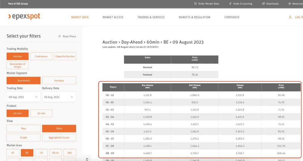
Instead, we have to scrape the data from the website. Luckily, I’m not the first person to do this. I found this GitHub repository where Steffen Zimmermann already went through the hassle of analyzing the website’s HTML code and extracting the data we need from it. By looking at that source code and taking the bits and pieces we need from it, we can achieve the same result in a Notebook.

Installing beautifulsoup4

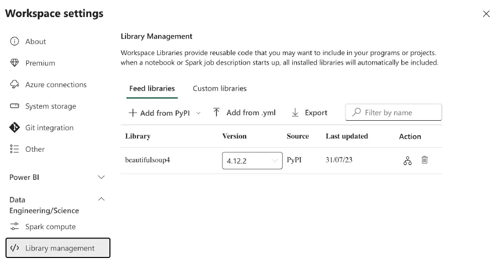
Before we can get started, we first need to install the beautifulsoup4 Python package in the Spark runtime environment of our Fabric Workspace. This can be done by going to your Workspace settings and then expanding the Data Engineering/Science section. There, you will find the </> Library management tab. Click on it and then on the + Add from PyPI button. In the text box that appears, enter beautifulsoup4, pick the latest version, and click on the Apply button. This will install the package in your Workspace. I suggest you take a coffee now since the installation process took a few minutes for me.

The Notebook

Now it’s time to have some fun and start playing with the data. Create a new Notebook and follow Fabric’s prompts to also create a new Lakehouse. Both operations take a few seconds and don’t require any infrastructure to be provisioned.

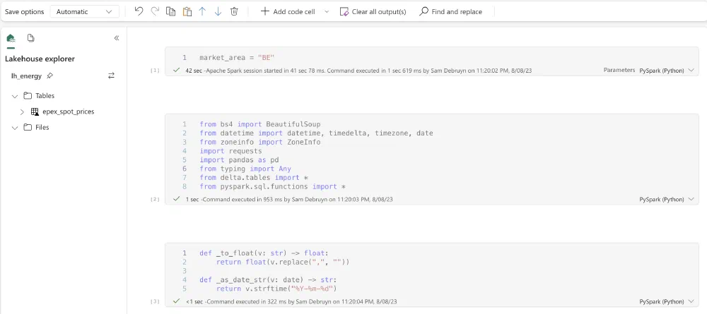
Unfortunately the Fabric feature to export Notebooks doesn’t fully work yet, so I cannot share the Notebook itself at the time of writing. I will update this post with a link to a downloadable version you can import once this feature is available. In the meantime, the code below is the full Notebook. Let’s go through it step by step.

  1market_area = "BE"
  2
  3from datetime import date, datetime, timedelta, timezone
  4from typing import Any
  5
  6import pandas as pd
  7import requests
  8from bs4 import BeautifulSoup
  9from delta.tables import *
 10from pyspark.sql.functions import *
 11
 12
 13def _to_float(v: str) -> float:
 14    return float(v.replace(",", ""))
 15
 16def _as_date_str(v: date) -> str:
 17    return v.strftime("%Y-%m-%d")
 18
 19def extract_invokes(data: dict[str, Any]) -> dict[str, Any]:
 20    invokes = {}
 21    for entry in data:
 22        if entry["command"] == "invoke":
 23            invokes[entry["selector"]] = entry
 24    return invokes
 25
 26def fetch_data(delivery_date: date, market_area: str) -> dict[str, Any]:
 27    trading_date = delivery_date - timedelta(days=1)
 28    params = {
 29        "market_area": market_area,
 30        "trading_date": _as_date_str(trading_date),
 31        "delivery_date": _as_date_str(delivery_date),
 32        "modality": "Auction",
 33        "sub_modality": "DayAhead",
 34        "product": "60",
 35        "data_mode": "table",
 36        "ajax_form": 1,
 37    }
 38    data = {
 39        "form_id": "market_data_filters_form",
 40        "_triggering_element_name": "submit_js",
 41    }
 42    r = requests.post("https://www.epexspot.com/en/market-data", params=params, data=data)
 43    r.raise_for_status()
 44    return r.json()
 45
 46def extract_table_data(delivery_date: datetime, data: dict[str, Any], market_area: str) -> pd.DataFrame:
 47    soup = BeautifulSoup(data["args"][0], features="html.parser")
 48
 49    try:
 50        table = soup.find("table", class_="table-01 table-length-1")
 51        body = table.tbody
 52        rows = body.find_all_next("tr")
 53    except AttributeError:
 54        return []  # no data available
 55
 56    start_time = delivery_date.replace(hour=0, minute=0, second=0, microsecond=0)
 57
 58    # convert timezone to UTC (and adjust timestamp)
 59    start_time = start_time.astimezone(timezone.utc)
 60
 61    records = []
 62    for row in rows:
 63        end_time = start_time + timedelta(hours=1)
 64        buy_volume_col = row.td
 65        sell_volume_col = buy_volume_col.find_next_sibling("td")
 66        volume_col = sell_volume_col.find_next_sibling("td")
 67        price_col = volume_col.find_next_sibling("td")
 68        records.append(
 69            (
 70                market_area,
 71                start_time,
 72                end_time,
 73                _to_float(buy_volume_col.string),
 74                _to_float(sell_volume_col.string),
 75                _to_float(volume_col.string),
 76                _to_float(price_col.string),
 77            )
 78        )
 79        start_time = end_time
 80
 81    return pd.DataFrame.from_records(records, columns=["market", "start_time", "end_time", "buy_volume", "sell_volume", "volume", "price"])
 82
 83def fetch_day(delivery_date: datetime, market_area) -> pd.DataFrame:
 84    data = fetch_data(delivery_date.date(), market_area)
 85    invokes = extract_invokes(data)
 86
 87    # check if there is an invoke command with selector ".js-md-widget"
 88    # because this contains the table with the results
 89    table_data = invokes.get(".js-md-widget")
 90    if table_data is None:
 91        # no data for this day
 92        return []
 93    return extract_table_data(delivery_date, table_data, market_area)
 94
 95current = DeltaTable.forName(spark, "epex_spot_prices")
 96current_df = current.toDF()
 97current_df = current_df.withColumn("date", to_date(col("start_time")))
 98current_market_count = current_df.filter((current_df.market == market_area) & (current_df.date == _as_date_str(datetime.now() + timedelta(days=1)))).count()
 99if current_market_count == 24:
100    mssparkutils.notebook.exit("Already ingested")
101
102prices = fetch_day(datetime.now() + timedelta(days=1), market_area)
103if len(prices) == 0:
104    mssparkutils.notebook.exit("No prices available yet")
105
106spark_df = spark.createDataFrame(prices)
107
108current.alias("current").merge(spark_df.alias("new"), "current.market = new.market AND current.start_time = new.start_time AND current.end_time = new.end_time").whenNotMatchedInsertAll().execute()

Walkthrough

Parameter cell

1market_area = "BE"

The first cell is a parameter cell where we set the market we want to ingest. I would like to run this notebook for all markets where Epex Spot is active, so by parametrizing the market area, we can pass the market area as a parameter to the notebook when we run it.

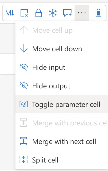
To make a cell a parameter cell, click on the ... next to the code cell and select Toggle parameter cell.

Imports

Next, we import all required libraries.

1from datetime import date, datetime, timedelta, timezone
2from typing import Any
3
4import pandas as pd
5import requests
6from bs4 import BeautifulSoup
7from delta.tables import *
8from pyspark.sql.functions import *

• Pandas is used to create a DataFrame from the data we extract from the website.
• Requests is used to make the HTTP request to the website.
• BeautifulSoup is used to parse the HTML response.
• Delta is used to write the data to the Delta table with the upsert functionality.
• And finally, we import some functions from the PySpark library to see if we already ingested the data and avoid extra HTTP requests and CU consumption (read more about billing in my previous blog post ).

Scraping functions

 1def _to_float(v: str) -> float:
 2    return float(v.replace(",", ""))
 3
 4def _as_date_str(v: date) -> str:
 5    return v.strftime("%Y-%m-%d")
 6
 7def extract_invokes(data: dict[str, Any]) -> dict[str, Any]:
 8    invokes = {}
 9    for entry in data:
10        if entry["command"] == "invoke":
11            invokes[entry["selector"]] = entry
12    return invokes
13
14def fetch_data(delivery_date: date, market_area: str) -> dict[str, Any]:
15    trading_date = delivery_date - timedelta(days=1)
16    params = {
17        "market_area": market_area,
18        "trading_date": _as_date_str(trading_date),
19        "delivery_date": _as_date_str(delivery_date),
20        "modality": "Auction",
21        "sub_modality": "DayAhead",
22        "product": "60",
23        "data_mode": "table",
24        "ajax_form": 1,
25    }
26    data = {
27        "form_id": "market_data_filters_form",
28        "_triggering_element_name": "submit_js",
29    }
30    r = requests.post("https://www.epexspot.com/en/market-data", params=params, data=data)
31    r.raise_for_status()
32    return r.json()
33
34def extract_table_data(delivery_date: datetime, data: dict[str, Any], market_area: str) -> pd.DataFrame:
35    soup = BeautifulSoup(data["args"][0], features="html.parser")
36
37    try:
38        table = soup.find("table", class_="table-01 table-length-1")
39        body = table.tbody
40        rows = body.find_all_next("tr")
41    except AttributeError:
42        return []  # no data available
43
44    start_time = delivery_date.replace(hour=0, minute=0, second=0, microsecond=0)
45
46    # convert timezone to UTC (and adjust timestamp)
47    start_time = start_time.astimezone(timezone.utc)
48
49    records = []
50    for row in rows:
51        end_time = start_time + timedelta(hours=1)
52        buy_volume_col = row.td
53        sell_volume_col = buy_volume_col.find_next_sibling("td")
54        volume_col = sell_volume_col.find_next_sibling("td")
55        price_col = volume_col.find_next_sibling("td")
56        records.append(
57            (
58                market_area,
59                start_time,
60                end_time,
61                _to_float(buy_volume_col.string),
62                _to_float(sell_volume_col.string),
63                _to_float(volume_col.string),
64                _to_float(price_col.string),
65            )
66        )
67        start_time = end_time
68
69    return pd.DataFrame.from_records(records, columns=["market", "start_time", "end_time", "buy_volume", "sell_volume", "volume", "price"])

The next 5 functions are used to scrape the data from the website. You can skip to the next paragraph if you are not that interested in the scraping itself. The code above basically works as follows:

1. We submit an HTTP POST request (a submitted form) to the web page and the server responds with a JSON object. The request has to contain the parameters that the users would normally select on the website.
2. Deeply nested inside this JSON object we get back, we find HTML code containing the table that contains the data we are interested in.
3. We pass the HTML code to BeautifulSoup, which parses the HTML code for us and we ask it to look for for the table.

The interesting part is located at the end of the code snippet above. Here, we loop over all rows in the table and append each of them to a list of tuples. We also convert the date and time to UTC, so that we don’t have to worry about timezones or daylight-saving time later on. Finally, we convert the list of tuples to a Pandas DataFrame.

 1def fetch_day(delivery_date: datetime, market_area) -> pd.DataFrame:
 2    data = fetch_data(delivery_date.date(), market_area)
 3    invokes = extract_invokes(data)
 4
 5    # check if there is an invoke command with selector ".js-md-widget"
 6    # because this contains the table with the results
 7    table_data = invokes.get(".js-md-widget")
 8    if table_data is None:
 9        # no data for this day
10        return []
11    return extract_table_data(delivery_date, table_data, market_area)

The last scraping-related function adds more error handling. It is not known when the pricing data becomes available, so the notebook will run multiple times a day until we have data for the next day.

First run & partitioning strategy

1prices = fetch_day(datetime.now() + timedelta(days=1), market_area)
2if len(prices) == 0:
3    mssparkutils.notebook.exit("No prices available yet")
4
5spark_df = spark.createDataFrame(prices)
6
7spark_df.write.mode("overwrite").format("delta").option("overwriteSchema", "true").partitionBy("market").saveAsTable("epex_spot_prices")

The code above is the version of the notebook that should be used on the very first run to initialize the Delta table. We call our scraping functions to fetch data for the market set above for the next day and then convert the Pandas DataFrame to a Spark DataFrame. We then write the Spark DataFrame to the Delta table.

The line mssparkutils.notebook.exit("No prices available yet") tells the notebook to exit gracefully, without errors, if the prices are not available yet.

The last line is the most interesting one. We write the data to the Delta table and partition it by market. This means that the data will be stored in multiple folders, one for each market. The folder structure will look like this:

 1epex_spot_prices
 2|── _delta_log
 3├── market=AT
 4│   ├── part-00000-....parquet
 5│   ├── part-00001-....parquet
 6│   ├── ...
 7├── market=BE
 8│   ├── part-00000-....parquet
 9│   ├── part-00001-....parquet
10│   ├── ...
11├── ...

Delta tables are locked when they are written to, except when the multiple processes are not writing to the same partition. So partitioning by market allows us to run the notebook concurrently for different markets.

Subsequent runs

1current = DeltaTable.forName(spark, "epex_spot_prices")
2current_df = current.toDF()
3current_df = current_df.withColumn("date", to_date(col("start_time")))
4current_market_count = current_df.filter((current_df.market == market_area) & (current_df.date == _as_date_str(datetime.now() + timedelta(days=1)))).count()
5if current_market_count == 24:
6    mssparkutils.notebook.exit("Already ingested")

On subsequent runs, we should avoid doing unnecessary HTTP calls by first checking if we already have the data for this market for the next day. Since there is one row per hour, we should have 24 rows per market. We can check this by counting the number of rows for the market and date we are interested in. If we have 24 rows, we can exit the notebook.

In the code above, I am loading the data first as a DeltaTable object so that we can use this later on to merge the new data with the existing data. I then convert the DeltaTable to a Spark DataFrame and add a column with the date. Then I filter the DataFrame to only contain the rows for the market and date we are interested in and count the number of rows.

1prices = fetch_day(datetime.now() + timedelta(days=1), market_area)
2if len(prices) == 0:
3    mssparkutils.notebook.exit("No prices available yet")
4
5spark_df = spark.createDataFrame(prices)
6
7current.alias("current").merge(spark_df.alias("new"), "current.market = new.market AND current.start_time = new.start_time AND current.end_time = new.end_time").whenNotMatchedInsertAll().execute()

Finally, we fetch the data for the next day and convert it to a Spark DataFrame. We then merge the new data with the existing data. The merge function is a Delta-specific function that allows us to merge two DataFrames. We merge the new data with the existing data on the columns market, start_time and end_time. We use the whenNotMatchedInsertAll function to insert all rows from the new DataFrame that do not match any rows in the existing DataFrame. This means that we will only insert the new rows. The execute function executes the merge operation.

This is where the magic of Delta Lake comes into play. Thanks to its transaction log, this merge or upsert operation becomes available. Doing the same thing with plain Parquet or CSV files would be much more difficult.

Since we have the check above, we could just ignore the merging and always append all new data, but years of data engineering have taught me that it is better to be safe than sorry.

The result

Now it’s time to run the notebook and see it in action. I’m always amazed by how fast Fabric can spin up a Spark session. The same operation took minutes with the platforms that were available a few years ago.

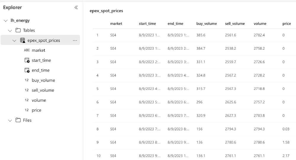
After running the notebook, you can find the Delta table in the Lakehouse.

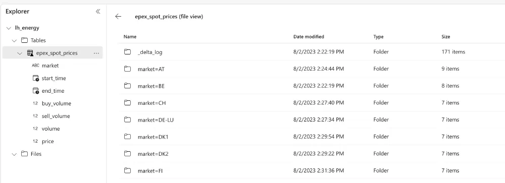
We can also check out the files by clicking on the ... and choosing View files. Here we see the partitioning strategy in action.

👉 Next part

In the next part, we’ll use our Notebook in a Pipeline and schedule it to run a couple of times a day.

The link will start working as soon as the post is published, about a week after this one.

You might also like

If you liked this article, follow me on LinkedIn or other social media to stay up-to-date with my latest posts. You might also like the following 2 posts about related topics:

Let Fabric teach you how to code with Data Wrangler

6 minutes

August 9, 2023

I’m going to be honest with you. I’m bad at writing Pandas data transformation code. Throughout the years I mostly focussed on the Spark APIs in Scala and PySpark, SQL, dbt, and some others, but I find the Pandas APIs usually just confusing and hard to read. I don’t like the black box magic and lock-in of low-code solutions either. Did you know that Microsoft Fabric has the perfect middle ground for this? It’s called Data Wrangler. Let’s dive in!

Read more

Fabric end-to-end use case: overview & architecture

6 minutes

August 21, 2023

Welcome to the first part of a 5-part series on an end-to-end use case for Microsoft Fabric. This post will focus on the architecture overview of the use case. In this series, we will explore how to use Microsoft Fabric to ingest, transform, and analyze data using a real-world use case.

Read more